Drawing a line between two groups sounds simple. If points on one side are blue and points on the other side are pink, any rule-based program can handle it. But what happens when the boundary is not a straight line? What if blue and pink regions interleave in complex patterns?
Traditional if-else logic breaks down quickly. You would need to hardcode every curve and corner. Change the pattern and you start from scratch. Neural networks offer a different approach. They learn the boundary by looking at examples instead of following explicit rules.
This project became my first experiment with building a neural network from scratch. No TensorFlow. No libraries. Just JavaScript, math, and a canvas to visualize the results.
What It Does
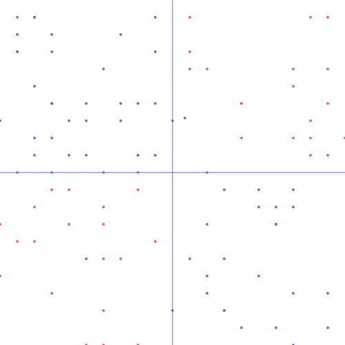
The application displays a 500x500 pixel canvas divided into colored zones. Blue occupies certain regions. Pink fills the others. The boundary between them follows a diagonal pattern based on two intersecting lines.
A hundred training points appear on the canvas. Blue dots mark blue zones. Pink dots mark pink zones. The neural network watches these examples and learns to classify any point you click.
Click anywhere on the canvas and the network predicts the zone. A new dot appears in blue or pink based on what the network thinks. Early predictions are random guesses. After training, predictions match the actual zones with high accuracy.
The error rate displays below the canvas. Watch it drop from near 50% to single digits as the network learns.
Clasificador de zonas
The Neural Network Architecture
The network has three layers with a simple topology: 4 neurons, then 2 neurons, then 1 output neuron.
Input comes as X and Y coordinates. These two values feed into the first hidden layer of 4 neurons. That layer passes to a second hidden layer of 2 neurons. The final output neuron produces a value between 0 and 1. Values closer to 1 predict blue. Values closer to 0 predict pink.
Each neuron multiplies its inputs by weights, adds a bias term, then applies a sigmoid activation function. The sigmoid squashes any value into the 0 to 1 range. This creates smooth transitions that work well for classification tasks.
How It Learns
The network uses backpropagation to adjust its weights. Here is the process:
- Forward pass - Input coordinates flow through each layer, producing an output prediction
- Calculate loss - The difference between predicted and actual class becomes the error
- Backward pass - The error propagates back through each layer
- Update weights - Each weight adjusts proportionally to how much it contributed to the error
The learning rate controls how big each adjustment is. Too high and the network overshoots. Too low and learning takes forever. This implementation uses 0.5, which converges quickly for this problem.
Every 300 milliseconds, the network runs through all training points. Each pass is one training iteration. The weights get a little better each time.
The Math Behind It
Forward propagation calculates the output of each layer. For a given input, the layer multiplies by its weight matrix, adds the bias vector, and applies sigmoid to each element.
The sigmoid function maps any real number to a value between 0 and 1:
f(x) = 1 / (1 + e^(-x))Its derivative has a convenient form that makes backpropagation efficient:
f'(x) = f(x) * (1 - f(x))Backpropagation works backwards from the output. At each layer, it computes how much each weight contributed to the error. The gradient tells us the direction of steepest increase. We subtract to move toward lower error.
The delta at each layer depends on two things: the derivative of the activation function and the error signal from the layer above. Matrix multiplication handles the weight updates efficiently.
Data Generation
Training data comes from a simple rule. Two invisible lines divide the plane. Points where both lines agree (both above or both below) belong to one class. Points where the lines disagree belong to the other.
The data generator creates 100 random points within a 20x20 unit square. For each point, it checks which side of each line the point falls on. The combination determines blue or pink.
This creates a pattern that a single straight line cannot separate. The network must learn a nonlinear boundary. That is why hidden layers matter. Each layer adds complexity to what the network can represent.
Visualization
The canvas renders at 500x500 pixels with the origin at the center. Each unit in the coordinate system maps to 25 pixels. A point at (2, 3) appears at pixel (300, 175).
Blue dots use the hex color #616aff. Pink dots use #ff566f. The axes draw in blue to provide reference. Training points appear as small circles. Click points appear at the same size.
The error display updates after each training iteration. It shows the average absolute error across all training points. Watching this number drop gives immediate feedback on learning progress.
Challenges
Getting backpropagation right took several attempts. Matrix dimensions must align perfectly. A single transpose in the wrong place breaks everything silently. The output looks plausible but never improves.
The first version updated weights incorrectly. Error decreased at first, then plateaued at 50%. Random chance. The network was not actually learning. Tracing through the math by hand revealed a missing derivative term.
Weight initialization also mattered. Starting weights too large caused neurons to saturate. Sigmoid outputs all 0s or all 1s, gradients vanish, learning stops. Initializing weights between -1 and 1 avoided saturation.
What I Learned
Building a neural network from scratch forces you to understand every piece. Matrix multiplication is not magic. Backpropagation is just calculus. The learning happens through simple arithmetic applied thousands of times.
Three layers with under 20 total neurons can learn surprisingly complex boundaries. Deep networks are not always necessary. For many problems, shallow networks work fine.
The most valuable insight was how gradients flow backward. Each layer’s error depends on the layers after it. This chain of dependencies is why we call it backpropagation. Understanding it at the math level made later work with modern frameworks much clearer.
This project also taught me that visualization makes debugging easier. Watching dots appear on a canvas shows immediately if predictions make sense. The error plot shows if learning is happening. Without visualization, I would have spent much longer tracking down bugs.